10.2 Short term
10.2.1 Goal
Decompose a short term time series of e.g. 5 days 15min data:
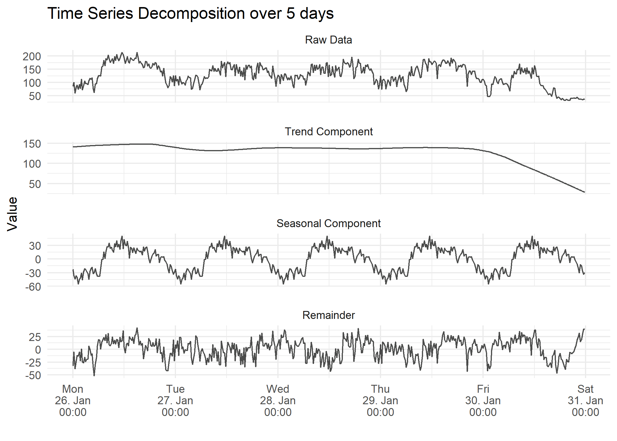
Figure 10.4: Seasonal Plot Overlapping per Month over 10 Years
10.2.2 Data Basis
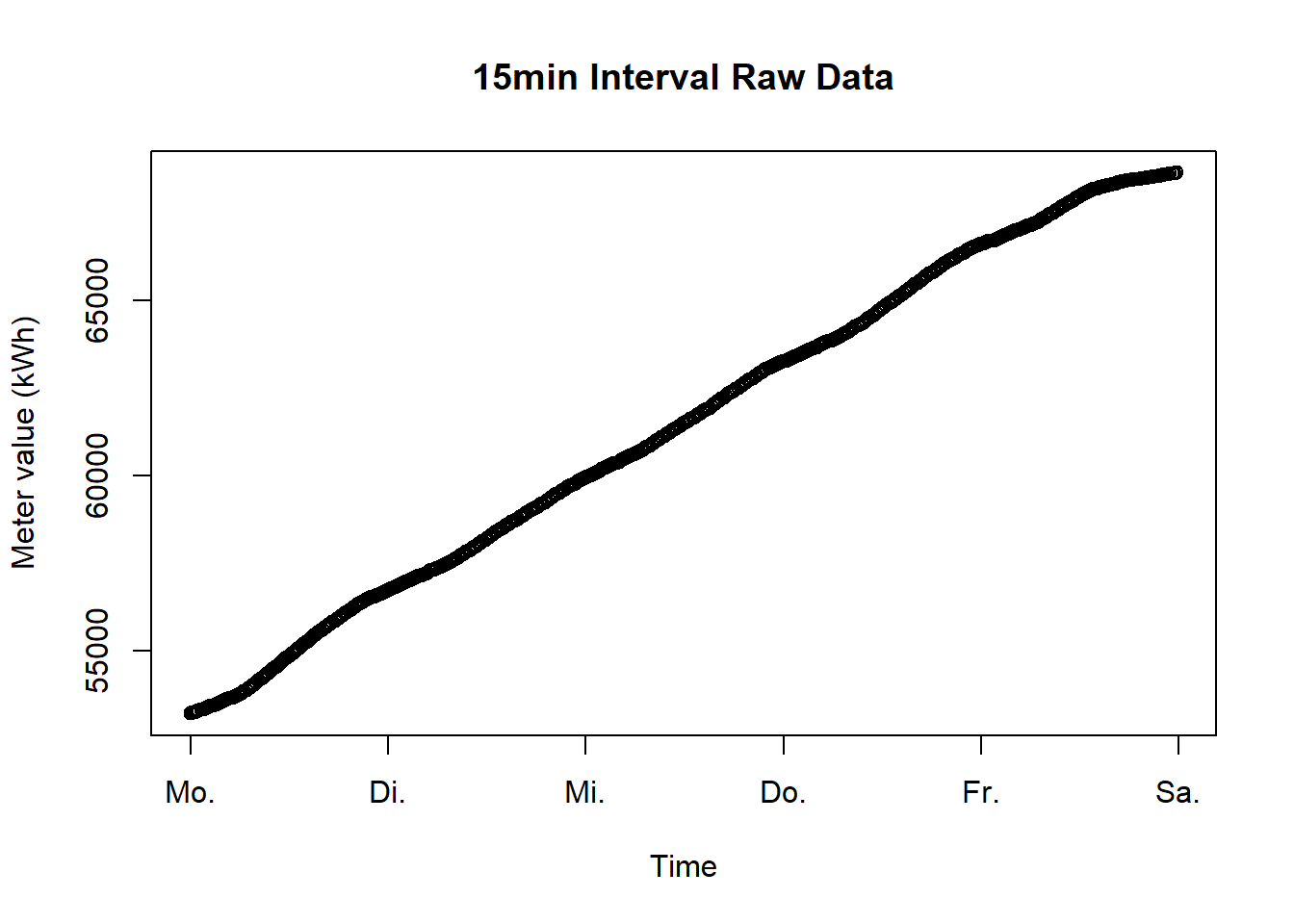
Figure 10.5: Raw Data for Decomposition Plot Short Term
10.2.3 Solution
Create a new script, copy/paste the following code and run it:
library(dplyr)
library(lubridate)
library(plotly)
library(ggplot2)
library(forecast)

# change language to English, otherwise weekdays are in local language
Sys.setlocale("LC_TIME", "English")
## [1] "English_United States.1252"# load time series data
df <- read.csv("https://github.com/hslu-ige-laes/edar/raw/master/sampleData/eboBookEleMeter.csv",
stringsAsFactors=FALSE,
sep =";")
# rename column names
colnames(df) <- c("time", "meterValue")
df$time <- parse_date_time(df$time,
orders = "YmdHMS",
tz = "Europe/Zurich")
df$time <- force_tz(df$time, tzone = "UTC")
# uncomment to filter time range if necessary
#df <- df %>% filter(Time > "2015-03-01 00:00:00", Time < "2015-04-01 00:00:00")
# Fill missing values with NA
grid.df <- data.frame(time = seq(min(df$time, na.rm = TRUE),
max(df$time, na.rm = TRUE),
by = "15 mins"))
df <- merge(df, grid.df, all = TRUE)
# convert steadily counting energy meter value from kWh to power in kW
df <- df %>%
dplyr::mutate(value = (meterValue - lag(meterValue))*4) %>%
select(-meterValue) %>%
na.omit()
# remove negative values which occur beause of change summer/winter time
df <- df %>% filter(value >= 0)
# select time range
df <- df %>% filter(time >= as.POSIXct("2015-01-26 00:00:00", tz = "UTC"),
time < as.POSIXct("2015-01-31 00:00:00", tz = "UTC"))
# =========== Start of Code ================
df.ts <- ts(df %>% select(value) %>% na.omit(),
frequency = 96)
df.decompose <- df.ts[,1] %>%
stl(s.window = 193)
df.decompose <- df.decompose$time.series
df.decompose <- as.data.frame(df.decompose)
df.decompose <- cbind(df, df.decompose)
data <- as.data.frame(tidyr::pivot_longer(df.decompose,
cols = -time,
names_to = "component",
values_to = "value",
values_drop_na = TRUE)
)
data$component <- as.factor(data$component)
data$component <- factor(data$component, c("value",
"trend",
"seasonal",
"remainder"))
# prepare data for plot
componentTitles = c("Raw Data","Trend Component", "Seasonal Component", "Remainder")
data <- data %>%
dplyr::mutate(component = recode(component,
value = componentTitles[1],
trend = componentTitles[2],
seasonal = componentTitles[3],
remainder = componentTitles[4]),
value = round(data$value, digits = 1)) %>%
rename(Value = value,
Time = time)
plot <- ggplot(data) +
geom_path(aes(x = Time,
y = Value
),
color = "black",
alpha = 0.7) +
facet_wrap(~component, ncol = 1, scales = "free_y") +
scale_x_datetime(date_breaks = "days" , date_labels = "%a\n%d. %b\n%H:%M") +
theme_minimal() +
theme(panel.spacing = unit(1, "lines"),
legend.position = "none") +
labs(x = "") +
ggtitle("Time Series Decomposition over 5 days")
ggplotly(plot)