16.4 Building Energy Signature Proposed
16.4.1 Goal
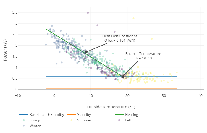
Create a plot of a building energy signature as proposed in “Development and validation of energy signature method”, Eriksson et al, 2020:

Figure 16.8: Building Energy Signature Plot “PES”
16.4.2 Data Basis

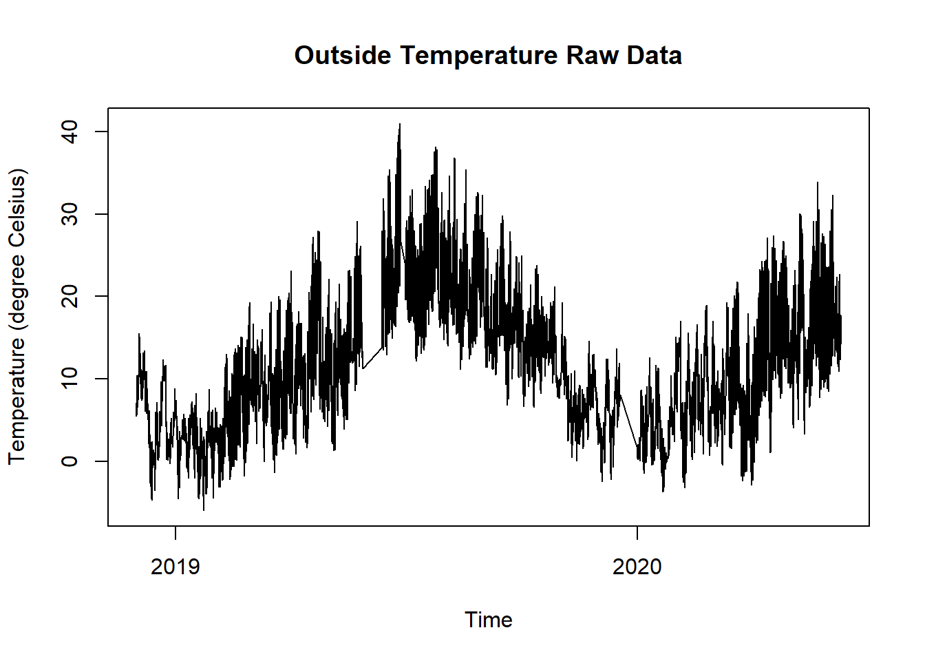
Figure 16.9: Energy Meter Raw Data for Building Energy Signature Plot

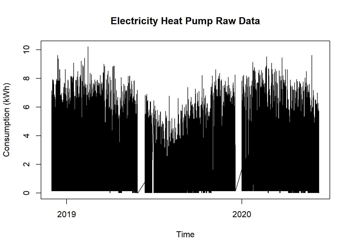
Figure 16.10: Energy Meter Raw Data for Building Energy Signature Plot

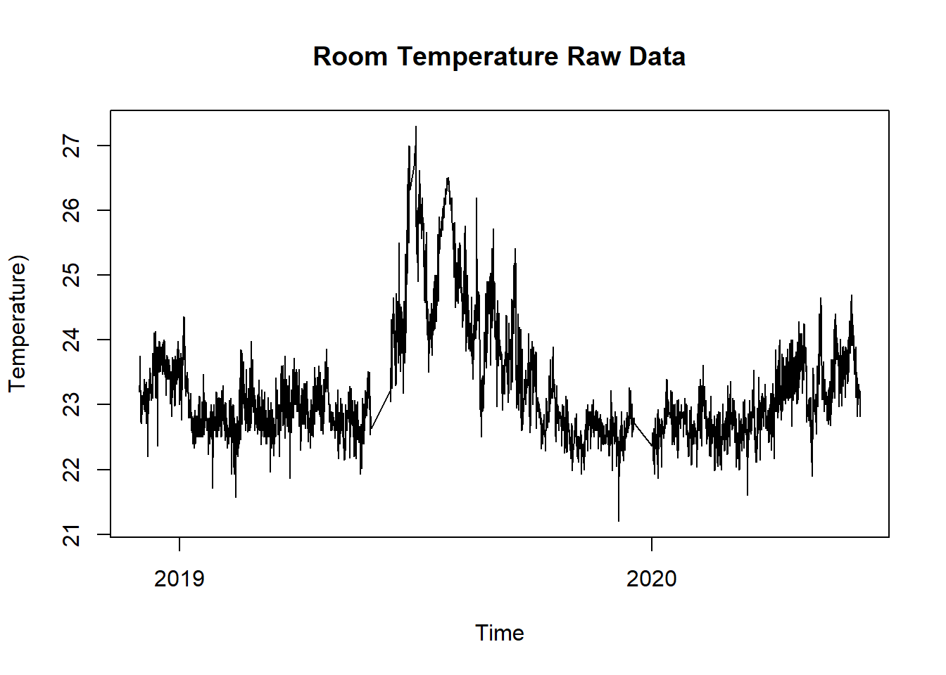
Figure 16.11: Energy Meter Raw Data for Building Energy Signature Plot
16.4.3 Solution
After reading in the two time series the data has to get aggregated per day and then merged. Note that during the aggregation of the energy data you have to calculate the daily conspumption from the steadiliy increasing meter values as well.
Create a new script, copy/paste the following code and run it:
library(plotly)
library(plyr)
library(lubridate)
library(redutils)

df.all <- read.csv("https://github.com/hslu-ige-laes/edar/raw/master/sampleData/bldgEngySigProposedData.csv",
                    stringsAsFactors=FALSE,
                    sep =",")

names(df.all)[1] <- "time"
names(df.all)[2] <- "TOa"
names(df.all)[3] <- "Energy"
names(df.all)[4] <- "TRoom"

df.all$time <- as.POSIXct(df.all$time,
                format="%Y-%m-%dT%H:%M:%OSZ", tz="Europe/Zurich")

df.all <- df.all %>%
  dplyr::mutate(season = getSeason(time),
                day = lubridate::date(time),
                month = lubridate::month(time),
                week = lubridate::week(time),
                hour = lubridate::hour(time),
                power = Energy
                ) %>%
  na.omit()

# Initial Balance Temperature Tb
Tb <- 12

# Initial difference
delta <- 1

while(abs(delta) > 0.1){

  # calculate standby power pStby
  # conditions
  # - TOa > Tb
  df <- df.all %>% group_by(week) %>%
    dplyr::mutate(keep = (mean(TOa, na.rm = TRUE) > Tb),
                  pStby = min(power, na.rm = TRUE)) %>%
    filter(keep == TRUE) %>%
    select(-Energy)

  pStby <- mean(df$pStby, na.rm = TRUE)

  # calculate hotwater power pHw
  # conditions
  # - TOa > Tb
    df <- df.all %>%
    group_by(week) %>%
    dplyr::mutate(keep = (mean(TOa, na.rm = TRUE) > Tb)) %>%
    dplyr::mutate(pHw = mean(power, na.rm = TRUE)) %>%
    filter(keep == TRUE)

  pHw <- mean(df$pHw, na.rm = TRUE) - pStby

  # Assumption for internal heat gains
  pIhg <- 3*90*9/1000/4.5  # 3 W/m^2, 90m^2/flat, 9 flats, COP WP 4.5, 24 hours per day

  # calculate internal heat generation pIhg
  # conditions
  # - Month is Jan, Feb and March
  # - TOa < Tb
  df <- df.all %>%
    filter(month %in% c(1,2,3)) %>%
    group_by(day) %>%
    dplyr::mutate(keep = (max(TOa, na.rm = TRUE) < Tb)) %>%
    filter(keep == TRUE) %>%
    dplyr::mutate(meanPower = mean(power, na.rm = TRUE)) %>%
    dplyr::mutate(meanTOa = mean(TOa, na.rm = TRUE))  %>%
    dplyr::mutate(meanTRoom = mean(TRoom, na.rm = TRUE)) %>%
    select(day, meanPower, meanTOa,  meanTRoom, week) %>%
    unique()

  # calculate Building total heat loss coefficient QTot in kW/K
  df <- df %>%
    dplyr::mutate(QTot = (meanPower - pStby - pHw + pIhg)/(meanTRoom - meanTOa))

  QTot <- mean(df$QTot, na.rm = TRUE)

  result <- NULL

  # Iterative determination of balance temperature Tb
  for(i in seq(10,30,0.1)){
    df.i <- df.all %>%
      dplyr::mutate(tempDiff = i - TOa) %>%
      filter(tempDiff > 0)

    df.i <- df.i %>%
      dplyr::mutate(powerCalc = (QTot * tempDiff + pStby + pHw))

    percDiff <- 100/sum(df.all$power, na.rm = TRUE) * sum(df.i$powerCalc, na.rm = TRUE)

    result = rbind(result, data.frame(Tb = i,
                                      percDiff = percDiff,
                                      power = sum(df.all$power),
                                      powerCalc = sum(df.i$powerCalc)))
  }

  Tb.new <- result[which(abs(result$percDiff-100) == min(abs(result$percDiff - 100), na.rm = TRUE)),1]
  delta <- Tb - Tb.new
  Tb <- Tb.new

}

# create plot
df <- df.all %>%
  group_by(day) %>%
  dplyr::mutate(TOaMean = mean(TOa, na.rm = TRUE)) %>%
  dplyr::mutate(powerSum = mean(power, na.rm = TRUE)) %>%
  select(day, TOaMean, powerSum, season) %>%
  na.omit() %>%
  unique() %>%
  ungroup()

names(df)[2] <- "TOa"
names(df)[3] <- "Power"

# df <- df %>% dplyr::mutate((EnergyHeat = TOa * -0.04955 + 4.5865) * Energy)
# names(df)[5] <- "EnergyHeat"

df.fall <- df %>% filter(season=="Fall")
df.winter <- df %>% filter(season=="Winter")
df.spring <- df %>% filter(season=="Spring")
df.summer <- df %>% filter(season=="Summer")

# annotations
a_Tb <- list(
  x = Tb,
  y = pStby + pHw,
  text = paste0("Balance Temperature<br> Tb = ",
                round(Tb, digits = 1),
                " \u00B0C"
                ),
  showarrow = TRUE,
  arrowhead = 7,
  ax = 70,
  ay = -70
)

a_QTot <- list(
  x = (Tb-min(df$TOa, na.rm = TRUE))/2+min(df$TOa, na.rm = TRUE),
  y = (Tb-min(df$TOa, na.rm = TRUE)) * QTot/2+pStby + pHw,
  text = paste0("Heat Loss Coefficient<br>QTot = ",
                round(QTot, digits = 3),
                " kW/K"),
  showarrow = TRUE,
  arrowhead = 2,
  ax = 120,
  ay = -50
)

# Create plot
p <- plot_ly()

p <- p %>% add_lines(x = c(min(df$TOa, Tb, na.rm = TRUE),max(df$TOa, na.rm = TRUE)),
                     y = rep((pStby + pHw), 2),
                     name = "Base Load + Standby",
                     hoverinfo = "text",
                     text = ~ paste("Base Load + Standby:  ", sprintf("%.3f kW", pStby + pHw)
                     ))
p <- p %>% add_lines(x = c(min(df$TOa, Tb, na.rm = TRUE), max(df$TOa, na.rm = TRUE)),
                     y = rep(pStby, 2),
                     name = "Standby",
                     hoverinfo = "text",
                     text = ~ paste("Standby:  ", sprintf("%.3f kW", pStby)
                     ))
p <- p %>% add_lines(x = c(min(df$TOa, na.rm = TRUE), Tb),
                     y = c((Tb-min(df$TOa, na.rm = TRUE)) * QTot + pStby + pHw, pStby + pHw), name = "Heating")

p <- p %>% add_markers(data = df.spring,
                       x = ~TOa,
                       y = ~Power,
                       marker = list(color = "#2db27d", opacity = 0.3),
                       name = "Spring",
                       hoverinfo = "text",
                       text = ~ paste("Outside Temp:  ", sprintf("%.1f \u00B0C", TOa),
                                      "<br />Power:  ", sprintf("%.1f kW", Power),
                                      "<br />Date:     ", day,
                                      "<br />Season: ", df.spring$season
                       )
  )

p <- p %>% add_markers(data = df.summer,
                       x = ~TOa,
                       y = ~Power,
                       marker = list(color = "#fde725", opacity = 0.3),
                       name = "Summer",
                       hoverinfo = "text",
                       text = ~ paste("Outside Temp:  ", sprintf("%.1f \u00B0C", TOa),
                                      "<br />Power:  ", sprintf("%.1f kW", Power),
                                      "<br />Date:     ", day,
                                      "<br />Season: ", df.summer$season
                       )
  )


p <- p %>% add_markers(data = df.fall,
                       x = ~TOa,
                       y = ~Power,
                       marker = list(color = "#440154", opacity = 0.3),
                       name = "Fall",
                       hoverinfo = "text",
                       text = ~ paste("Outside Temp:  ", sprintf("%.1f \u00B0C", TOa),
                                      "<br />Power:  ", sprintf("%.1f kW", Power),
                                      "<br />Date:     ", day,
                                      "<br />Season: ", df.fall$season
                       )
  )

p <- p %>% add_markers(data = df.winter,
                       x = ~TOa,
                       y = ~Power,
                       marker = list(color = "#365c8d", opacity = 0.3),
                       name = "Winter",
                       hoverinfo = "text",
                       text = ~ paste("Outside Temp:  ", sprintf("%.1f \u00B0C", TOa),
                                      "<br />Power:  ", sprintf("%.1f kW", Power),
                                      "<br />Date:     ", day,
                                      "<br />Season: ", df.winter$season
                       )
  )

p <- p %>%
  layout(
    xaxis = list(title = "Outside temperature (\u00B0C)", range = c(min(-10,min(df.all$TOa)), max(35,max(df.all$TOa))), zeroline = F),
    yaxis = list(title = "Power (kW)", range = c(min(df$Power, max(df$Power)))),
    showlegend = TRUE,
    legend = list(orientation = "h",
                  y = -0.2,
                  x = 0),
    annotations = list(a_Tb,a_QTot)
  ) %>%
  plotly::config(modeBarButtons = list(list("toImage")), displaylogo = FALSE)

p
16.4.4 Discussion
This is a new method, which calculates the balance Temperture, a heating loss coefficient in kW/K, a basic consumption (blue line) and a standby value (orange line) from 15min consumption data of an electric or heat meter in an iterative procedure using the outside and room temperature.