6.3 Examples

The following example show how these concepts can be applied in practice.

6.3.1 tidy up flatTempHum.csv

6.3.1.1 Loading data and parsing timestamp

library(tidyverse)
library(lubridate)

# load test data set
df <- read.csv("https://github.com/hslu-ige-laes/edar/raw/master/sampleData/flatTempHum.csv",
               stringsAsFactors=FALSE,
               sep =";")
df$time <- parse_date_time(df$time, "YmdHMS", tz = "Europe/Zurich")

head(df, 5)

##                  time FlatA_Hum FlatA_Temp FlatB_Hum FlatB_Temp FlatC_Hum
## 1 2018-10-03 00:00:00      53.0      24.43      38.8      22.40      44.0
## 2 2018-10-03 01:00:00      53.0      24.40      38.8      22.40      44.0
## 3 2018-10-03 02:00:00      53.0      24.40      39.3      22.40      44.7
## 4 2018-10-03 03:00:00      53.0      24.40      40.3      22.40      45.0
## 5 2018-10-03 04:00:00      53.3      24.40      41.0      22.37      45.2
##   FlatC_Temp FlatD_Hum FlatD_Temp
## 1       24.5      49.0      24.43
## 2       24.5      49.0      24.40
## 3       24.5      48.3      24.38
## 4       24.5      48.0      24.33
## 5       24.5      47.7      24.30

6.3.1.2 tidy up

What needs to be done here to get this data set into a tidy format?

Firstly each observation should have its own row… To fulfill that, we have to convert from wide to long.
Secondly, the variables are flat and sensor which are currently merged together in the column name. That must be separated.

# convert wide to long format
df.long <- as.data.frame(tidyr::pivot_longer(df,
                                             cols = -time,
                                             names_to = "datapoint",
                                             values_to = "value",
                                             values_drop_na = TRUE))
head(df.long, 5)

##         time  datapoint value
## 1 2018-10-03  FlatA_Hum 53.00
## 2 2018-10-03 FlatA_Temp 24.43
## 3 2018-10-03  FlatB_Hum 38.80
## 4 2018-10-03 FlatB_Temp 22.40
## 5 2018-10-03  FlatC_Hum 44.00

# separate datapoint into two columns
df.separated <- df.long %>% 
  separate(col = datapoint, into = c("flat", "sensor"), sep = "_") %>% 
  mutate_at("flat", str_replace, "Flat", "") %>% 
  na.omit()

head(df.separated, 10)

##                   time flat sensor value
## 1  2018-10-03 00:00:00    A    Hum 53.00
## 2  2018-10-03 00:00:00    A   Temp 24.43
## 3  2018-10-03 00:00:00    B    Hum 38.80
## 4  2018-10-03 00:00:00    B   Temp 22.40
## 5  2018-10-03 00:00:00    C    Hum 44.00
## 6  2018-10-03 00:00:00    C   Temp 24.50
## 7  2018-10-03 00:00:00    D    Hum 49.00
## 8  2018-10-03 00:00:00    D   Temp 24.43
## 9  2018-10-03 01:00:00    A    Hum 53.00
## 10 2018-10-03 01:00:00    A   Temp 24.40

This dataset can now be considered tidy and is ready for further processing.

6.3.1.3 convert to ‘tsibble’

library(tsibble)

# convert the data frame in a tsibble object
tsbl <- as_tsibble(df.separated, key = c(flat, sensor), index = time)
tsbl

## # A tsibble: 131,602 x 4 [1h] <Europe/Zurich>
## # Key:       flat, sensor [8]
##    time                flat  sensor value
##    <dttm>              <chr> <chr>  <dbl>
##  1 2018-10-03 00:00:00 A     Hum     53  
##  2 2018-10-03 01:00:00 A     Hum     53  
##  3 2018-10-03 02:00:00 A     Hum     53  
##  4 2018-10-03 03:00:00 A     Hum     53  
##  5 2018-10-03 04:00:00 A     Hum     53.3
##  6 2018-10-03 05:00:00 A     Hum     53.7
##  7 2018-10-03 06:00:00 A     Hum     50.8
##  8 2018-10-03 08:00:00 A     Hum     42.7
##  9 2018-10-03 09:00:00 A     Hum     46  
## 10 2018-10-03 10:00:00 A     Hum     41.3
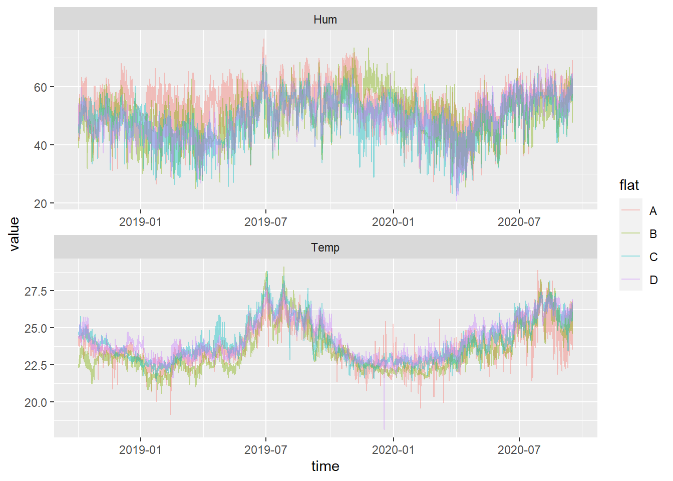
## # ... with 131,592 more rows

6.3.1.4 Visualization

It’s now relatively easy and straightforward to make a plot using the key-columns flat and sensor:

library(ggplot2)

ggplot(tsbl, aes(x= time, y= value, colour = flat)) +
  geom_line(alpha=0.4) +
  facet_wrap(~ sensor,  scales="free", ncol = 1)