13.1 Overview

13.1.1 Goal

Create an overview of typical daily profiles per weekday and season of year with a confidence band where most of the values lie:

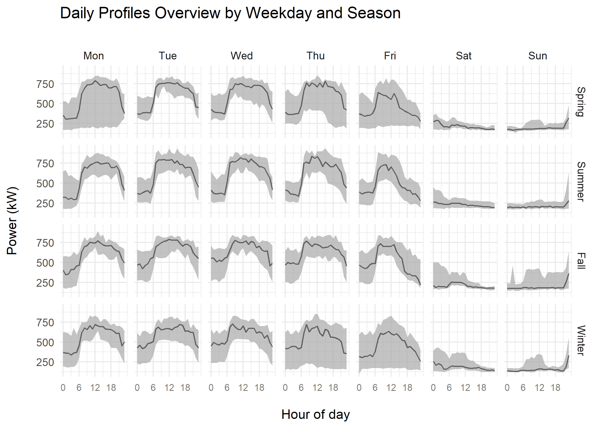
Figure 13.1: Overview of Daily Profiles by Weekday and Season

13.1.2 Data Basis

Energy consumption values of one whole year in an interval of 15mins.

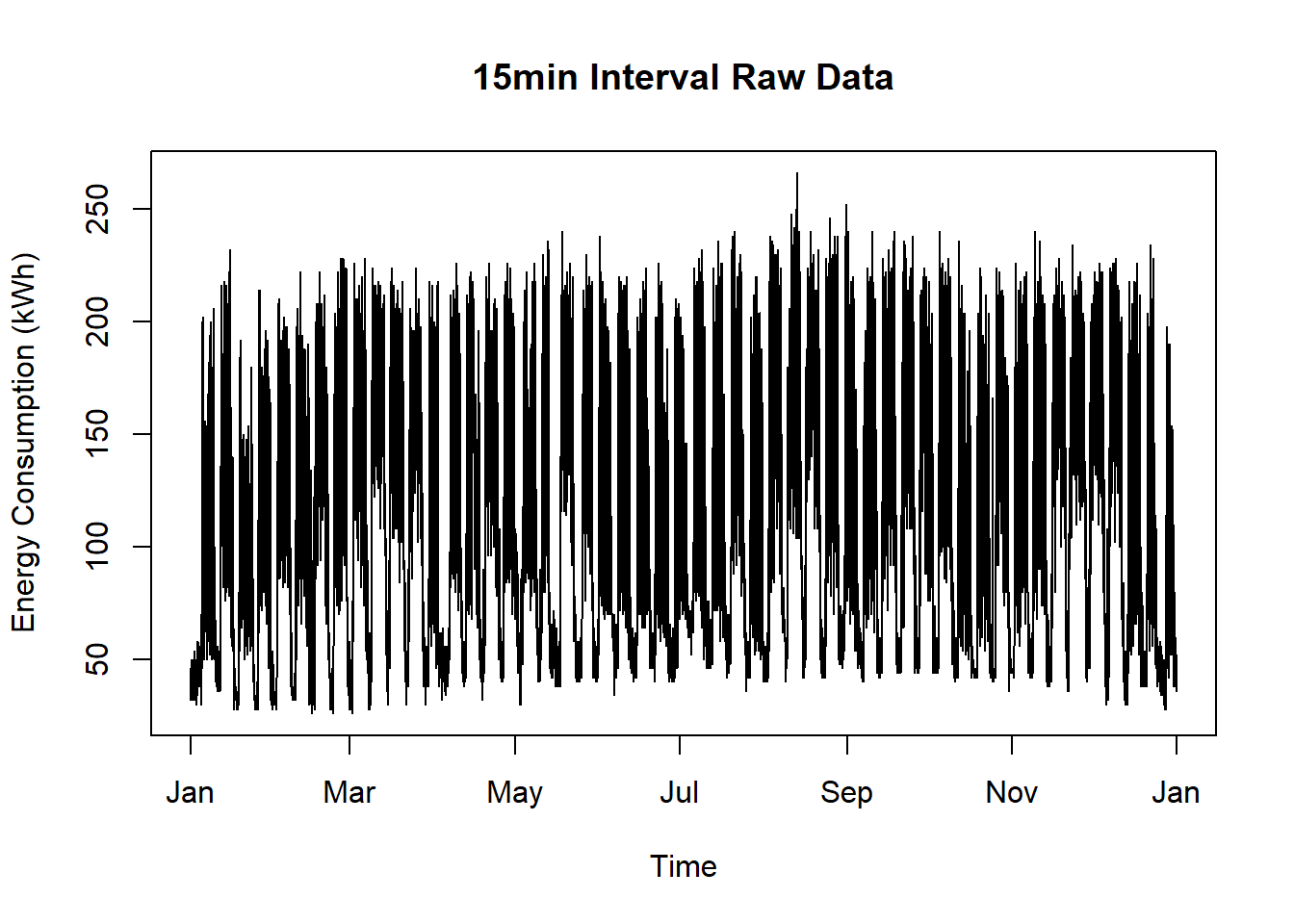
Figure 13.2: Raw Data for Decomposition Plot Short Term

13.1.3 Solution

Create a new script, copy/paste the following code and run it:

library(ggplot2)
library(dplyr)
library(lubridate)
library(redutils)
library(ggplot2)
library(plotly)

# load time series data
df <- readRDS(system.file("sampleData/eboBookEleMeter.rds", package = "redutils"))

plot <- plotDailyProfilesOverview(df,
                               locTimeZone = "Europe/Zurich",
                               main = "Daily Profiles Overview by Weekday and Season",
                               ylab = "Power (kW)",
                               col = "black",
                               confidence = 95.0)

ggplotly(plot)

# save static plot as png (optional)
ggsave("images/plotDailyProfOverview.png", plot)